
User Guide: Difference between revisions
| (42 intermediate revisions by the same user not shown) | |||
| Line 19: | Line 19: | ||
*c) '''Open''': Open an existing file. The result of this operation depends on the contents of the file being opened. There are some file naming conventions, but the name itself is not used to determine the type of file. There are four main types of files that can be opened: GIS raster map files, SELES static model files, SELES dynamic model files and SELES scenario files. These files are each opened by selecting the desired file using the browser. Information on the internal structure of these SELES files is described in other documents. | *c) '''Open''': Open an existing file. The result of this operation depends on the contents of the file being opened. There are some file naming conventions, but the name itself is not used to determine the type of file. There are four main types of files that can be opened: GIS raster map files, SELES static model files, SELES dynamic model files and SELES scenario files. These files are each opened by selecting the desired file using the browser. Information on the internal structure of these SELES files is described in other documents. | ||
The GIS formats supported are GRASS (binary, compressed and ASCII), ERDAS (8 and 16 bit) and ARC ASCII. To open a GIS raster map file, select the raster file in a GIS database to open (for GRASS this will be a file in the “cell” directory of a mapset). The map contained in this file (in conjunction with information stored in associated files, such as the header and colour files) will be displayed in a new window. | *:The GIS formats supported are GRASS (binary, compressed and ASCII), ERDAS (8 and 16 bit) and ARC ASCII. To open a GIS raster map file, select the raster file in a GIS database to open (for GRASS this will be a file in the “cell” directory of a mapset). The map contained in this file (in conjunction with information stored in associated files, such as the header and colour files) will be displayed in a new window. | ||
*:There are four types of static model files (See the section on the Static Models Menu and the SELES Static Model Reference for more details). | |||
There are four types of static model files (See the section on the Static Models Menu and the SELES Static Model Reference for more details). | |||
**(i) '''SELES Neutral Model Files''' (generally with a .nm suffix) contain information for creating neutral models. Provided that a valid model is read, a new view is opened and an instance of the model is generated. | **(i) '''SELES Neutral Model Files''' (generally with a .nm suffix) contain information for creating neutral models. Provided that a valid model is read, a new view is opened and an instance of the model is generated. | ||
**(ii) '''SELES Site Specific Model Files''' (generally with a .sm suffix) contain information for creating site-specific models. Provided that a valid model is read, and that the views required by this model exist, a new view is opened and an instance of the model is generated. | **(ii) '''SELES Site Specific Model Files''' (generally with a .sm suffix) contain information for creating site-specific models. Provided that a valid model is read, and that the views required by this model exist, a new view is opened and an instance of the model is generated. | ||
**(iii) '''SELES Fractal Model Files''' (generally with a .frm suffix) contain information for creating fractal models. Provided that a valid model is read, a new view is opened and an instance of the model is generated. | **(iii) '''SELES Fractal Model Files''' (generally with a .frm suffix) contain information for creating fractal models. Provided that a valid model is read, a new view is opened and an instance of the model is generated. | ||
**(iv) '''SELES Value Model Files''' (generally with a .vm suffix) contain information for creating Value (or Statistical Summary) Models. Provided that a value model is read, and that the views required by this model exist, an instance of the model is generated. | **(iv) '''SELES Value Model Files''' (generally with a .vm suffix) contain information for creating Value (or Statistical Summary) Models. Provided that a value model is read, and that the views required by this model exist, an instance of the model is generated. | ||
*:SELES Simulation Model Files (generally with a .sel suffix) are used to organize and store a complete specification of a dynamic landscape simulation model. Provided a valid simulation model is read, and that the views containing the initial conditions for the simulation exist, the simulation is set up. This set-up reads in and checks the landscape events used by the model, and initializes the initial state of all raster layers. Any views for displaying the output state of dynamic layers are automatically created, if required. | |||
*:SELES Scenario Files (generally with a .scn suffix) are used to group a set of GIS and model files. When opened, each sub-model file listed in the scenario file will be loaded in the order specified. This is useful, for example, to load a set of GIS raster layers that form the initial conditions for a simulation and a SELES Simulation Model. | |||
*d) '''DryRun''': Opens and “dry runs” a scenario file. A dry run performs all tasks in a scenario except for actually running a simulation. | |||
* | *e) '''Close''': Close the current selected view. This can also be accomplished by clicking with the mouse on the “Close” icon (the “X”) on the top right corner of the view window. | ||
* | *f) '''CloseAll''': Close all views and documents. | ||
* | *g) '''Save''': This option is the same as Save As. | ||
* | *h) '''Save As ...''': Save the raster in the currently active view as a GIS raster file or the | ||
currently displayed image in the view as a JPEG file. This option will bring up a file browser from which the directory and file name can be set. The “Save as type” pull-down menu allows selection of the type of information or GIS format to save. The directory for a GRASS GIS raster should be the “cell” directory of a GRASS mapset. The header and other required associated files will be automatically created in the correct directory of the mapset. | currently displayed image in the view as a JPEG file. This option will bring up a file browser from which the directory and file name can be set. The “Save as type” pull-down menu allows selection of the type of information or GIS format to save. The directory for a GRASS GIS raster should be the “cell” directory of a GRASS mapset. The header and other required associated files will be automatically created in the correct directory of the mapset. | ||
* | *i) '''List of recent documents''': Between the print options and the Exit option is a list of the recently opened documents (if any). A document can be re-opened or the window associated with a currently opened document can be activated by selecting from this list. | ||
* | *j) '''Exit''': Exit the SELES application. This can also be achieved by clicking with the mouse on the “Close” icon (the “X”) on the top right corner of the main application window. | ||
==View Menu== | ==View Menu== | ||
| Line 106: | Line 104: | ||
*a) '''Neutral Model''': Neutral models are a generalization of the neutral landscape models introduced by Gardner, O’Neill, Turner, et al. The original neutral models only permitted two feature types; we have generalized these to any number of features. Essentially, a neutral model is a description of the characteristics (or constraints) of a pattern that are independent of other (i.e. external) ecological and abiotic patterns and processes. An instance of a neutral model is a single map (layer) that is produced using these constraints. We have also improved the manner in which contagion is computed during model generation (removing the high levels of horizontal bias in the Gardner et al. models). | *a) '''Neutral Model''': Neutral models are a generalization of the neutral landscape models introduced by Gardner, O’Neill, Turner, et al. The original neutral models only permitted two feature types; we have generalized these to any number of features. Essentially, a neutral model is a description of the characteristics (or constraints) of a pattern that are independent of other (i.e. external) ecological and abiotic patterns and processes. An instance of a neutral model is a single map (layer) that is produced using these constraints. We have also improved the manner in which contagion is computed during model generation (removing the high levels of horizontal bias in the Gardner et al. models). | ||
*:To produce instances of a neutral model, set up the constraints, as described below, and press the Generate button. When finished, the dialog can be closed with “Cancel”. | |||
To produce instances of a neutral model, set up the constraints, as described below, and press the Generate button. When finished, the dialog can be closed with “Cancel”. | *:[[Image:Neutral model.gif]] | ||
*:The following are the constraints that can be used to express a neutral model: | |||
[[Image:Neutral model.gif]] | |||
The following are the constraints that can be used to express a neutral model: | |||
**i) '''Width''': The number of columns (cells per row) in the neutral model raster. | **i) '''Width''': The number of columns (cells per row) in the neutral model raster. | ||
**ii) '''Height''': The number of rows (cells per column) in the neutral model raster. | **ii) '''Height''': The number of rows (cells per column) in the neutral model raster. | ||
| Line 123: | Line 118: | ||
**x) '''Use Old Model''': If selected, produce model instances using an older algorithm. The older algorithm exhibits a "stripping" bias when high levels of contagion are specified. | **x) '''Use Old Model''': If selected, produce model instances using an older algorithm. The older algorithm exhibits a "stripping" bias when high levels of contagion are specified. | ||
**xi) '''Load from File/Save to File''': Load model parameters from or save to the file specified in the adjacent text box. These files generally should have a .nm suffix. It is useful to load pre-existing model files, modify them to suit the current needs and then save these to a new file. These neutral model files can be opened directly using the Open menu item in the Files menu described in section II. | **xi) '''Load from File/Save to File''': Load model parameters from or save to the file specified in the adjacent text box. These files generally should have a .nm suffix. It is useful to load pre-existing model files, modify them to suit the current needs and then save these to a new file. These neutral model files can be opened directly using the Open menu item in the Files menu described in section II. | ||
*b) '''Fractal Model''': Fractal models are landscape pattern models generated using a stochastic mid-point replacement algorithm, based on Mandelbrot’s fractal geometry. A number of controls are provided to influence various aspects of the pattern generation process. In addition, the values for zero or more fixed control points can be specified to “pin” down the landscape at various locations. These fractal landscape pattern models often exhibit characteristics similar elevation maps, and thus are often used as synthetic digital terrain models (DEMs). | |||
*:To produce instances of a fractal model, set up the constraints, as described below, and press the Generate button. When finished, the dialog can be close with the Cancel button. | |||
*:The following are the constraints that can be used to express a fractal model: | |||
**i) '''Width''': The number of columns (cells per row) in the fractal model raster. | |||
**ii) '''Height''': The number of rows (cells per column) in the fractal model raster. | |||
**iii) '''Number of Features''': The maximum number of features ("elevation" values) that may occur in an instance. | |||
**iv) '''Minimum Feature''': The numeric value of the "lowest" feature in the model (generally 0 or 1). | |||
**v) '''Fractal Degree''': Controls the degree of fine-scaled variability in the fractal model. | |||
**vi) '''Fractal Ratio''': Controls the rate of decline in variability as details are filled in. | |||
**vii) '''Concavity Threshold''': Specifies the threshold at which a pair of adjacent triangles is considered to represent a concave feature of the landscape. | |||
**viii)'''Concavity Slope''': Specifies the degree to which concave features have less variability than other features of the landscape (this is to avoid having valley bottoms with excessive “lakes” produced by a high fractal degree needed to make ridge tops more variable. | |||
**ix) '''Reseed''': If set, then the random number generator is reseeded with its previous seed value when the model instance is produced. This will cause the same instance to be produced again. If this option is not set, then a different instance will be produced. | |||
**x) '''Random Triangulation''': If set, then the triangulation decomposition process of the fractal model generation will be purely random; otherwise this decomposition process is regular. For the moment, use only regular decomposition. | |||
**xi) '''Colour Display''': If selected, then instances of the model will be displayed in colour. Otherwise they will be displayed in black and white. | |||
**xii) '''Clear Control Points''': Clear (delete) the current set of cell value control points. | |||
**xiii) '''Add Control Point''': Add to the current list of cell value control points the cell specified by Row and Col, and with a value specified by Value. In instance generation, this cell will be guaranteed to have the value specified. In this way, the overall coarse-scale structure of the landscape produced can be controlled. The more points that are specified, the more this fixed structure exerts an influence on the instances generated. | |||
**xiv) '''Load From''': Load model parameters from the file specified in the adjacent text box. These files generally should have a .frm suffix. It is useful to load pre-existing model files, modify them to suit the current needs and then save these to a new file. However, at the moment, there is not save facility; one must edit .frm files using a text editor. These fractal model files can be opened directly using the Open menu item in the Files menu described in section II. | |||
*c) '''Site (Specific) Model''': Site models generalize neutral models by allowing the relative probabilities of features to vary according to site characteristics. That is, a function in the form of a cell expression is evaluated at each site (raster cell), computing a relative probability for each feature at a site (this may be thought of as defining a fundamental niche for the feature). These probabilities are multiplied by the static probabilities specified in the dialog box to determine the final relative probabilities for each feature (analogous to the realized niche). The cell expression can depend on other information layers, such as elevation, aspect, soil, etc. For example, the relative proportion of a feature may increase with elevation. This type of model is very similar to a GIS raster overlay. | |||
*:As for neutral models, there can be any number of features. Also, a site model is a description of the characteristics (or constraints) of a layer that may be dependent on other (i.e. external) ecological and abiotic patterns and processes in a landscape. An instance of a site model is a single map (layer) that is produced using these constraints. Contagion can also be used to “clump” features more or less than they would occur at random, although the spatial structure of input layers on which the model is dependent may also partially achieve this effect. | |||
*:To produce instances of a site model, set up the constraints, as described below, and press the Generate button. When finished, the dialog can be close “Cancel”. | |||
*:[[Image:GSSM.gif]] | |||
*:The following are the constraints that can be used to express a site model: | |||
**i) '''Width''': The number of columns (cells per row) in the site model raster. | |||
**ii) '''Height''': The number of rows (cells per column) in the site model raster. | |||
**iii) '''Number of Features''': The maximum number of features (landscape element types) that may occur in an instance. | |||
**iv) '''Minimum Feature''': The numeric value of the first feature (generally 0 or 1). | |||
**v) '''Number of Start Points''': This is used in conjunction with contagion. It specifies the number of locations that are to be independently chosen (i.e. without using contagion). It must be at least one, but may be any positive number. These points are selected randomly in the output map. The remaining cells are produced using the influence of contagion and previously computed cell values. | |||
**vi) '''Cell Expression''': The file name of a cell expression to evaluate for computing the site-specific relative probabilities. | |||
**vii) '''Relative Abundance of Features''': The site independent relative abundance (i.e. relative probability) of each of the first seven features. These represent the expected relative occurrence of each feature in the landscape, in the absence of other spatial information. At a given site, the relative probabilities returned by the cell expression are multiplied by these static probabilities to produce a final set of relative probabilities for the site. Where contagion is used (especially high values of contagion), the actual abundance may be quite different. In this situation, these represent the expected relative occurrence of each feature over all instances of the model. Note that the relative abundance specified for feature 7 applies to all features greater than 7 (i.e. it applies to features in the range [7, Number of Features]. | |||
**viii) '''Colour Display''': If selected, then instances will be displayed in colour. Otherwise they will be displayed in black and white. | |||
**ix) '''Use Contagion''': If selected, then contagion is used to generate model instances. Contagion represents the degree to which features in the landscape are grouped together. A contagion value of 0 means no contagion (i.e. adjacency of features is random), while a value of 1 means that the probability of adjacent cells having the same value is 1. Values of contagion between zero and one cause varying degrees of "clumping" or spatial autocorrelation. | |||
**x) '''Contagion''': The value of contagion to use. Currently, the value can only be in the range [0,1]. | |||
**xi) '''Use Old Model''': If selected, produce model instances using an older algorithm. The older algorithm exhibits a "stripping" bias when high levels of contagion are specified. | |||
**xii) '''Variable and Viewname drop-down lists''': the names of the views (windows) for layer variables used by the cell expression. For example, if the cell expression requires a layer variable called “topography”, then this variable will appear in the Variables list. This will map to view that contains topography in the Viewnames list. | |||
**xiii) '''Load from File/Save to File''': Load model parameters from or save to the file specified in the adjacent text box. These files generally should have a .sm suffix. It is useful to load pre-existing model files, modify them to suit the current needs and then save these to a new file. These site model files can be opened directly using the Open menu item in the Files menu described in section II. | |||
*d) '''Value (or Statistical Summary) Model''': Value (or summary) models produce a single value by summarizing a function (specified as a cell expression) that computes a value for each cell in the landscape. The resulting value is displayed in the dialog box when “Generate” is pressed. | |||
*:To compute a value model, set up the function, as described below, and press the Run button to compute from an input file or RunEdits to compute from the expression written in the edit box. When finished, the dialog can be close with the Cancel button. | |||
*:The following parameters can be used to express a value model: | |||
**i) '''Operation''': Chose the desired summary function: mean, minimum value, maximum value, sum over all values, product over all values, nth root over all values (where n is the number of values computed). | |||
**ii) '''Cell Expression''': The file name of a cell expression to evaluate for computing the value for each site. | |||
**iii) '''Region''': The region is always the entire landscape. The edit box associated with the region allows users to specify a decision to limit the computation to a specific portion of the landscape. | |||
**iv) '''Variable and Viewname drop-down lists''': the names of the views (windows) for layer variables used by the cell expression. For example, if the cell expression requires a layer variable called “topography”, then this variable will appear in the Variables list. This will map to view that contains topography in the Viewnames list. When opened, all current views are automatically linked to variables of the same name. | |||
**v) '''Cell Expression Edit box''': This box allows users to type in an arbitrary cell expression, and can be used much like a console for querying or modifying the landscape state. | |||
*e) '''Align Layer''': The Align Layer feature aligns the currently selected layer with the layer chosen in the “Align with Layer” drop-down list by matching their georeferencing. If the layers are already aligned, no action is performed. If the layers are not aligned, then a new view is created with the name “alignedMAP”, where "MAP" is the name of the view chosen to align. The georeferencing of the new view will match the view chosen in the “Align with Layer” drop-down list. The contents of the new view will be the original view clipped to the new georeferencing. Any cells within the clip region, but not covered by the original layer will have a value of zero. | |||
*:Models in SELES must be aligned to run properly. That is, all raster layers must have the same extent (number of rows and columns) and must represent the same geographic location. This permits simulations to access all relevant information for a cell with a single location index. | |||
*:Once the layer to align with has been selected, the top-left and bottom-right bounds of the original image are shown relative to the georeferencing of the “Align with Layer”. These are called the aligned bounds. Any portion of the layer outside the range of the "Align with Layer" is clipped. Once an appropriate "Align with Layer" has been selected, the operation is performed by pressing the OK button. | |||
*f) '''Resize Layer''': The Resize Layer feature allows a raster to be resized, without changing its resolution. The dialog allows users to enter new bounds (top, left, bottom, right) for the raster. When the OK button is pushed, a new view with the same name but prefixed with “Resized” is created for the resized raster. | |||
==Dynamic Models Menu== | |||
There are three types of dynamic models available from this menu, a dialog box for setting up dynamic output of layers, and a dialog box for controlling simulations. Dynamic models generally produce a series of model instances or, in the case of Dynamic Value Models, a series of values, during the course of a simulation. All three dynamic models (Dynamic Site Model, Dynamic Value Model, Seles Model) may depend on other layers in the current scenario. | |||
*a) '''Dynamic Site Model''': A Dynamic Site Model is a site model that is re-computed periodically during a simulation. Since these models may depend on dynamically changing layers in the scenario, periodic recomputation of the model may produce different results. | |||
*:The dialog is identical to the static Site Model dialog except for an “Output Frequency” option. The value specified (in days and years) determines how often the site model is to be recomputed. For example, a value of 2 years will cause the model to be recomputed every 730.5 days or unit time steps. If the output frequency is zero, then the site model will be recomputed every time an event occurs during the simulation. If the output frequency is negative, then the model will be recomputed every time one of the parameter layers is modified. This may be useful if one or more of the parameter layers are being changed by an external model. | |||
*b) '''Dynamic Value Model''': A Dynamic Value Model is a value model that is re-computed periodically during a simulation. Since these models may depend on one or more dynamically changing layers in the scenario, periodic updating may produce different results. The dialog is similar to the static Value Model dialog with two additional options. | |||
*:[[Image:DSSVMG.gif]] | |||
**i) '''Output Filename''': If the “Save Output to File” option is chosen, then the output will be stored in the named file. Each run (of a Monte Carlo simulation) will be stored on a different line, and each output value will be separated by a tab character. This allows the model output to be loaded into a spreadsheet (e.g. Excel) for post-mortem analysis. | |||
**ii) '''Output Frequency''': The value specifies how often the model is to be recomputed during a simulation. If the output frequency is zero, then the model will be recomputed every time an event occurs during the simulation. If the output frequency is negative, then the model will be recomputed every time one of the parameter layers is modified. | |||
*c) '''Model Output''': Model Output allows intermediate states of dynamic layers to be saved during a simulation. The "Output Frequency" species how often the currently selected layer is to be saved. Each time the raster layer is saved, a new file is created with a unique filename: "BaseName#r.#s", where "BaseName" is the base filename, "#r" is the Monte Carlo run number, and "#s" is the sequence number for layer in this run. The “Filename Base or Directory” specifies where the raster layers are to be saved. If this names an existing directory, then the name of the currently selected layer will be used as the base filename, otherwise it specifies the full path and filename to be used as the base filename. For example, during run 2 with a filename base of “./results/test”, the sequence of files will be: './results/test2.1', './results/test2.2', etc. The available output types are uncompressed and compressed GRASS binary and GRASS ASCII, ERDAS 8 and 16 bit and ARC ASCII. Model output is set up by pressing the OK button, and terminated by pressing the Stop Output button. | |||
*:[[Image:Output control.gif]] | |||
*d) '''Seles Model''': A SELES Model specifies the information required to set up a simulation: that is, the input layers (initial spatial state), output layers (dynamic spatial state) and the landscape events. Once the information is entered or modified in the dialogue box, press “Setup” to prepare the model for simulation. This will not start a simulation – this is done using the Simulation Control dialog. | |||
*:[[Image:Setup seles models.gif]] | |||
*:The following parameters are used to express a SELES model: | |||
**i) '''Width and Height''': Specifies the spatial resolution as the number of columns and rows in the raster layers used by the scenario. | |||
**ii) '''Output Frequency''': The default frequency with which dynamic layers are updated on the screen. If the output frequency is zero, then the view for the dynamic layers will be refreshed every time an event occurs during a simulation. | |||
**iii) '''Landscape Event Filenames''': A drop-down list of the file names of landscape events used in the simulation. A SELES simulation requires one or more landscape events. The “Use Event” check box can be used to disable/enable specific events. | |||
**iv) '''Variables and Initial State Viewnames''': There is a (partial) mapping from layer variables in landscape events to viewnames that contain the initial spatial state of the variable. This mapping connects variables with their starting state raster layers at the beginning of a simulation or Monte-Carlo run. If the viewname is “<unassigned>”, then the initial state is assume to be a raster of zeros. | |||
**v) '''Variables and Output Viewnames''': There is a (partial) mapping from dynamic layer variables in landscape events to viewnames that contain the current (dynamic) spatial state of the variable. This mapping connects variables with the view in which the dynamic output layer for this variable is displayed during a simulation. If the viewname is “<unassigned>”, then the output state is not displayed (but will be maintained internally). | |||
**vi) '''Load from File/Save to File''': Load model parameters from or save to the file specified in the adjacent text box. These files generally should have a .sel suffix. It is useful to load pre-existing model files, modify them to suit the current needs and then save these to a new file. These SELES model files can be opened directly using the Open menu item in the Files menu described in section II. | |||
*e) '''Simulate''': This displays a dialog that provides the necessary functions to control simulations. Once all the dynamic models are set up, then the simulation scenario is ready to run. Since this dialog is modeless, other actions can be performed while the box is on the screen, and while a simulation is in progress. | |||
*:[[Image:Simulation control.gif]] | |||
*:The dialog allows control of a simulation as follows: | |||
**i) '''Simulation Length''': Specifies (in days and years) the length of time to run a simulation. “Current Time” is an output value that shows the current time of a running simulation. Note that a SELES model may use any unit timestep. For convenience, the unit timestep is called a "day" on the user interface, where one year = 365.25 days. If the unit timestep in your model is not a day, then read "Days" as "Unit Timesteps" on SELES dialogues. | |||
**ii) '''Runs''': Total: Specifies the number of Monte Carlo simulation runs. This can only be set before a simulation starts. “Runs: Current” is an output value that shows the current Monte Carlo run number. | |||
**iii) '''Output Frequency''': Specifies how often the model in the currently selected view is to be redisplayed. (See notes on unit timestep above.) | |||
**iv) '''Step Size''': Specifies how the number of time-steps to be made when “stepping through” a simulation. | |||
**v) '''Simulate''': Starts a simulation (or a complete series of Monte Carlo simulations). This button will change to a “Stop” during the simulation. Pressing “Stop” will terminate the simulation. | |||
**vi) '''Pause''': Allows a simulation to pause. While on pause, this button will change to a “Continue” button. Pressing “Continue” will resume the simulation. | |||
**vii) '''Step''': Allows a simulation to be "stepped through" in discrete time steps. If the simulation has not yet begun, then pressing this button will start it. Once the time period specified by “Step Size” has passed, the simulation will pause. At this point the “Pause” button will change to “Continue”. The user can press “Step” again to continue the simulation for “Step Size” time units, or press “Continue” to continue the simulation without stepping. Note that the Step button can be pressed at any time during a simulation to enter step mode. | |||
**viii) '''Cancel''': If a simulation is currently running, Cancel is the same as Stop. If a simulation is not running, then Cancel will close the Simulation Control Dialog. | |||
**ix) '''External Global Variables''': This is a list of global variables defined in landscape events. The initial state value of global variables is zero by default, but may be specified in a SELES Model file or dialogue. During a simulation, the values of dynamic variables are periodically updated in the dialog box. The current value of a global variable can be changed by selecting it in the scrollable list, typing a new value in the “Value” edit box and pressing “Set”. The initial state value of a variable can be similarly changed, pressing “Set Initial State” instead of “Set”. | |||
*f) '''Simulation Probe''': This option brings up a dialog box that allows probing of internal values in landscape events/agents during simulation. The desired event can be selected from a drop-down menu as well as the desired property context. Values for the agent/cell, cluster/group, event/population and cell variables are shown in different areas of the dialog. If changes occur too fast to see, there is an option to slow down the simulation. Care must be taken when using the probe, since it must modify events to operate. As a consequence, making too many changes on the dialog runs the risk of crashing a simulation due to timing of the user interface operation and the separate simulation engine processes. | |||
*g) '''Model Report''': This option saves a dynamic model report to two files called “SelesModelReport.txt” and “SelesModelReport2.txt” in the current directory. These files organizes all the layer and global variables, and global constants in the model state-space by type and lists the events that include them in their definitions section. The files also indicate if a variable or constant appears on the left-hand side (LHS), right-hand side (RHS), both or neither of an expression in the named event. The only difference between the files is format – the first is easier for browse while the second is more suitable for loading into a spreadsheet. This is useful for model verification, since at a glance it is easy to see variables that are not used, misspelled or not declared properly. Particular attention should be paid to variables that have no initial state. | |||
*h) '''Simulation Priority''': This option allows users to set the priority level for the simulation engine. On a single-processor machine (i.e. most desktops and laptops), decreasing the engine priority to Low or Lowest can increase responsiveness of the user interface and other programs. | |||
Latest revision as of 23:03, 3 November 2006
Note: this conversion between the Word .doc and the Wiki is incomplete: please help
Documentation Version SELES v3.1
The purpose of this guide is to assist users of the Windows version of SELES. The SELES user interface is based on Windows NT, and runs best under Windows NT, Windows 2000 and Windows XP. It assumes that the models to be used have already been constructed. See the SELES Model Builder’s Guide and the SELES Scenario Reference for information on how to construct SELES models. This document describes how to use the SELES program to load in initial conditions and models and to run simulations.
Startup
After starting SELES, the user will be presented with the following interface. The operations available under each pull down menu are described in the following sections.

File Menu
The file menu has the following options.
- a) New: Creates a new view window with a viewname “Seles#”, where # is a number (numbered sequentially from 1). The underlying raster will be 100 by 100, with all zeros.
- b) New2: Creates a new view window with dimensions taken from a current view, and user specified bounds and name. A pull down list of current views can be used to select the reference layer.
- c) Open: Open an existing file. The result of this operation depends on the contents of the file being opened. There are some file naming conventions, but the name itself is not used to determine the type of file. There are four main types of files that can be opened: GIS raster map files, SELES static model files, SELES dynamic model files and SELES scenario files. These files are each opened by selecting the desired file using the browser. Information on the internal structure of these SELES files is described in other documents.
- The GIS formats supported are GRASS (binary, compressed and ASCII), ERDAS (8 and 16 bit) and ARC ASCII. To open a GIS raster map file, select the raster file in a GIS database to open (for GRASS this will be a file in the “cell” directory of a mapset). The map contained in this file (in conjunction with information stored in associated files, such as the header and colour files) will be displayed in a new window.
- There are four types of static model files (See the section on the Static Models Menu and the SELES Static Model Reference for more details).
- (i) SELES Neutral Model Files (generally with a .nm suffix) contain information for creating neutral models. Provided that a valid model is read, a new view is opened and an instance of the model is generated.
- (ii) SELES Site Specific Model Files (generally with a .sm suffix) contain information for creating site-specific models. Provided that a valid model is read, and that the views required by this model exist, a new view is opened and an instance of the model is generated.
- (iii) SELES Fractal Model Files (generally with a .frm suffix) contain information for creating fractal models. Provided that a valid model is read, a new view is opened and an instance of the model is generated.
- (iv) SELES Value Model Files (generally with a .vm suffix) contain information for creating Value (or Statistical Summary) Models. Provided that a value model is read, and that the views required by this model exist, an instance of the model is generated.
- SELES Simulation Model Files (generally with a .sel suffix) are used to organize and store a complete specification of a dynamic landscape simulation model. Provided a valid simulation model is read, and that the views containing the initial conditions for the simulation exist, the simulation is set up. This set-up reads in and checks the landscape events used by the model, and initializes the initial state of all raster layers. Any views for displaying the output state of dynamic layers are automatically created, if required.
- SELES Scenario Files (generally with a .scn suffix) are used to group a set of GIS and model files. When opened, each sub-model file listed in the scenario file will be loaded in the order specified. This is useful, for example, to load a set of GIS raster layers that form the initial conditions for a simulation and a SELES Simulation Model.
- d) DryRun: Opens and “dry runs” a scenario file. A dry run performs all tasks in a scenario except for actually running a simulation.
- e) Close: Close the current selected view. This can also be accomplished by clicking with the mouse on the “Close” icon (the “X”) on the top right corner of the view window.
- f) CloseAll: Close all views and documents.
- g) Save: This option is the same as Save As.
- h) Save As ...: Save the raster in the currently active view as a GIS raster file or the
currently displayed image in the view as a JPEG file. This option will bring up a file browser from which the directory and file name can be set. The “Save as type” pull-down menu allows selection of the type of information or GIS format to save. The directory for a GRASS GIS raster should be the “cell” directory of a GRASS mapset. The header and other required associated files will be automatically created in the correct directory of the mapset.
- i) List of recent documents: Between the print options and the Exit option is a list of the recently opened documents (if any). A document can be re-opened or the window associated with a currently opened document can be activated by selecting from this list.
- j) Exit: Exit the SELES application. This can also be achieved by clicking with the mouse on the “Close” icon (the “X”) on the top right corner of the main application window.
View Menu
The main options available from this menu are “Raster View Properties”, “Show Legend” and “Histogram”. Show Legend brings up a dialog that displays legend information (taken from a GRASS-format “cats”, or category, file associated with a raster or model file) for the currently selected view. It also shows the colour, value and label under the mouse position.
Raster View Properties brings up the following dialog box to control image display properties. The “Colour Display” check box controls whether the image is output in colour or black and white. The “Raster Number” list is only used for multi-layer (interleaved) rasters. Each view of a multi-layer raster can select a single raster layer for display. The "Raster Value Range" is used to select an appropriate range of values for displaying these rasters. For ordinary rasters, the value range shows the minimum and maximum values for the raster and cannot be edited. The option “Fit Colours to Max/Min will rescale the colour lookup table to match the actual range of values rather than the bounds.

The “Use Image as Mask” option allows selection of another view to use as a visual mask on the current image. If selected, those values in the range [Minimum, Maximum] from the mask image will be drawn over the current layer.
The “Use Image as Hue” allows another image to be used as a hue modifier for the current image display. If selected, then the chosen view will be used to modify the hue of the current image. The minimum and maximum values from the chosen view should contain values that specify the minimum and maximum hue value in the hue image. Higher values in the hue image will cause the corresponding pixels in the current image to be displayed brighter.
The “Use Image as Depth” option allows an image to be displayed as a 3-D map, where the selected image provides the height, or elevation, of each pixel in the 3-D map. If selected, then the current image will be "draped" over the 3-D representation of the "Depth" image. There are two methods for rendering the 3-D representation of the height data. “Continuous” height data is used when the raster is a continuous variable (such as elevation), in which neighbouring values have similar in values, and are thus interpolated. “Discrete” height data is for rasters that represent a categorical variable, and so neighbouring height values are not assumed to be related.
This dialog box is also used to control the shared memory state of the image in a view. The default is for the image to be local. That is, the memory for the image is local and internal to the current SELES application. If “Offer Image to Share” is selected, then the image will be local to the current SELES application, but other applications that include SEED shared memory support can access the image directly. That is, an external application can “open” the shared memory image and access it as if the memory were local to that application. If “Share External Memory” is selected, then the image named in the “External Image Name” is assumed to have been offered by some external application with SEED shared memory support. If found, the image behaves as if it was local to this SELES application, but it will actually be in shared memory between the two applications.
The “Histogram” option brings up a dialog box with which simple histograms can be displayed of selected layers, optionally masked by other layers”. The colours used for the histogram classes are taken from the colour used for the smallest value in the class. The “Histogram2” option brings up a more detailed dialog box in which histograms can be specified as in summary models by defining the region over which the histogram is defined, and the function used to define classes.
Window Menu
The Window menu has the following options:
- a) New Window: Creates a new window with the same model or image as the currently active view. Different windows that refer to the same image have the same viewname, with a suffix consisting of a colon and a sequence number (e.g. Seles1:1 and Seles1:2).
- b) Cascade: Cascades the currently opened windows.
- c) Tile: Tiles the currently opened windows.
- d) Arrange Icons: No effect at the moment.
- e) Name Document: Allows user to change the name of the currently active view. This may be necessary to create a view of the appropriate name for a particular SELES model, since SELES models refer to images by their view names.
- f) Minimize All: Minimize all windows.
- g) Minimize Initial State: Minimize all windows that contain initial state information for the currently loaded dynamic model.
- h) Minimize Static: Minimize all windows that contain static information for the currently loaded dynamic model.
- i) List of current windows: The bottom portion of this menu contains a list of the windows that currently exist. The active window is shown with a check mark beside it. A window can be activated by selecting from this list (or by clicking on the window itself).
Help Menu
Brings up on-line SELES help, in a standard Windows format. In general, this help is out-of-date and the user guides are more current.
Exchange Menu
This menu contains options for the SEED image exchange facilities. For most users, these options are not relevant. The “Server Port” option opens the following dialog box:

The current port used by this application to “listen” for requests from clients is shown. If a different port is desired it can be changed. Pressing “OK” will attempt to change the listening port to the new port, and the dialog box will disappear. Pressing “Reset” will change the port back to the value it last had. Pressing “Cancel” will close the dialog and retain the current listening port.
The “Import Data” option opens the following dialog box. This dialog sets up communication with other SEED applications. In the simplest case, a single layer from a remote SEED application can be imported by pressing the “Import” button. To do this, one must know the machine name on the Internet and the port of the application on this machine. If the “Currently Active” document is selected, then the layer in the currently active window of the remote application will be imported. As a result of this operation, the layer in the remote application will be copied to the currently active window on the local SELES application.
If the port is unknown, a list of SEED applications and their port numbers can be obtained by pressing the “Ports on Server” button. Note that this operation can potentially be time consuming due to network timeouts for ports without SEED applications. The desired remote application can be chosen from the resulting list. Also, a remote server can be “tested” to see if it is a SEED application by pressing the “Test Server” button.

To browse and select from the active layers on a remote application, press the “Documents at Port” button. The layer to import can be selected from the resulting list. In addition to immediate import, the user can also request a layer to be imported each time it is updated by the remote server. If
“Image on Update” is selected, then the selected image in the external SEED application will be sent every time it is updated. In SELES, the action performed when a new image is received is to update the image in the window that was active when the command was invoked. If “Synchronous Update” is not selected, then the external SEED application will not wait for a reply when an updated image is sent. If it is selected, the external SEED application will await a reply from the current application for each image sent. Since SELES sends an acknowledging reply immediately, this option has no influence in this case. It is intended for SEED applications that wish to perform some other operation before replying (e.g. a harvest scheduler may wish to generate a new schedule to input to SELES before acknowledging receipt of an updated forest cover, thereby providing control to suspend SELES simulations).
“Cancel” will close the dialog without importing any image. If images are being received “On Update” to the currently active window, then “Cancel” will also stop this type of import.
Static Models Menu
There are five types of static models available from this menu. Static models generally produce a single model instance. Neutral and Fractal Models do not depend on other views in the current scenario, but Site and Value Models may use zero or more other views to produce their output. The "Align Layer" option on this menu is used to match the georeferencing of one layer based on a second layer.
See the Static Model Reference for more information on static models.
- a) Neutral Model: Neutral models are a generalization of the neutral landscape models introduced by Gardner, O’Neill, Turner, et al. The original neutral models only permitted two feature types; we have generalized these to any number of features. Essentially, a neutral model is a description of the characteristics (or constraints) of a pattern that are independent of other (i.e. external) ecological and abiotic patterns and processes. An instance of a neutral model is a single map (layer) that is produced using these constraints. We have also improved the manner in which contagion is computed during model generation (removing the high levels of horizontal bias in the Gardner et al. models).
- To produce instances of a neutral model, set up the constraints, as described below, and press the Generate button. When finished, the dialog can be closed with “Cancel”.
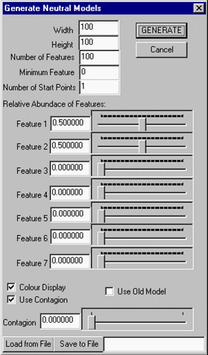
- The following are the constraints that can be used to express a neutral model:
- i) Width: The number of columns (cells per row) in the neutral model raster.
- ii) Height: The number of rows (cells per column) in the neutral model raster.
- iii) Number of Features: The maximum number of features (landscape element types) that may occur in an instance.
- iv) Minimum Feature: The numeric value of the first feature in the model (generally 0 or 1).
- v) Number of Start Points: This option is used in conjunction with contagion. It specifies the number of locations that are to be independently chosen (i.e. without using contagion). It must be at least one, but may be any number. These points are selected randomly in the output map. The remaining cells are produced using the influence of contagion from previously computed cell values.
- vi) Relative Abundance of Features: The relative abundance (i.e. relative probability) of each of the first seven features. These represent the expected relative occurrence of each feature in the landscape. Where contagion is used (especially high values of contagion), the actual abundance may be quite different. In this situation, these represent the expected relative occurrence of each feature over all instances of the model. Note that the relative abundance specified for feature 7 applies to all features greater than 7 (i.e. it applies to features in the range [7, Number of Features].
- vii) Colour Display: If selected, then instances will be displayed in colour. Otherwise they will be displayed in black and white.
- viii) Use Contagion: If selected, then contagion is used when model instances are generated. Contagion represents the degree to which features in the landscape are grouped together. A contagion value of 0 means no contagion (i.e. adjacency of features is random), while a value of 1 means that the probability of an adjacent cell having the same value is 1. Values of contagion between zero and one create varying degrees of "clumped" or spatially autocorrelated patterns. Negative contagion causes features of the same value to occur further apart than at random, where a value of -1 indicates that the probability of two adjacent cells holding the same feature is 0. Note that for extreme values of contagion (near -1 or 1), it may not be possible to simultaneously satisfy both the contagion constraints and the relative abundance constraints. We have proven a theorem that provides a method of coming as close as possible to satisfying both sets of constraints.
- ix)Contagion: The value of contagion to use. Currently, the value can only be in the range [0,1].
- x) Use Old Model: If selected, produce model instances using an older algorithm. The older algorithm exhibits a "stripping" bias when high levels of contagion are specified.
- xi) Load from File/Save to File: Load model parameters from or save to the file specified in the adjacent text box. These files generally should have a .nm suffix. It is useful to load pre-existing model files, modify them to suit the current needs and then save these to a new file. These neutral model files can be opened directly using the Open menu item in the Files menu described in section II.

- b) Fractal Model: Fractal models are landscape pattern models generated using a stochastic mid-point replacement algorithm, based on Mandelbrot’s fractal geometry. A number of controls are provided to influence various aspects of the pattern generation process. In addition, the values for zero or more fixed control points can be specified to “pin” down the landscape at various locations. These fractal landscape pattern models often exhibit characteristics similar elevation maps, and thus are often used as synthetic digital terrain models (DEMs).
- To produce instances of a fractal model, set up the constraints, as described below, and press the Generate button. When finished, the dialog can be close with the Cancel button.
- The following are the constraints that can be used to express a fractal model:
- i) Width: The number of columns (cells per row) in the fractal model raster.
- ii) Height: The number of rows (cells per column) in the fractal model raster.
- iii) Number of Features: The maximum number of features ("elevation" values) that may occur in an instance.
- iv) Minimum Feature: The numeric value of the "lowest" feature in the model (generally 0 or 1).
- v) Fractal Degree: Controls the degree of fine-scaled variability in the fractal model.
- vi) Fractal Ratio: Controls the rate of decline in variability as details are filled in.
- vii) Concavity Threshold: Specifies the threshold at which a pair of adjacent triangles is considered to represent a concave feature of the landscape.
- viii)Concavity Slope: Specifies the degree to which concave features have less variability than other features of the landscape (this is to avoid having valley bottoms with excessive “lakes” produced by a high fractal degree needed to make ridge tops more variable.
- ix) Reseed: If set, then the random number generator is reseeded with its previous seed value when the model instance is produced. This will cause the same instance to be produced again. If this option is not set, then a different instance will be produced.
- x) Random Triangulation: If set, then the triangulation decomposition process of the fractal model generation will be purely random; otherwise this decomposition process is regular. For the moment, use only regular decomposition.
- xi) Colour Display: If selected, then instances of the model will be displayed in colour. Otherwise they will be displayed in black and white.
- xii) Clear Control Points: Clear (delete) the current set of cell value control points.
- xiii) Add Control Point: Add to the current list of cell value control points the cell specified by Row and Col, and with a value specified by Value. In instance generation, this cell will be guaranteed to have the value specified. In this way, the overall coarse-scale structure of the landscape produced can be controlled. The more points that are specified, the more this fixed structure exerts an influence on the instances generated.
- xiv) Load From: Load model parameters from the file specified in the adjacent text box. These files generally should have a .frm suffix. It is useful to load pre-existing model files, modify them to suit the current needs and then save these to a new file. However, at the moment, there is not save facility; one must edit .frm files using a text editor. These fractal model files can be opened directly using the Open menu item in the Files menu described in section II.
- c) Site (Specific) Model: Site models generalize neutral models by allowing the relative probabilities of features to vary according to site characteristics. That is, a function in the form of a cell expression is evaluated at each site (raster cell), computing a relative probability for each feature at a site (this may be thought of as defining a fundamental niche for the feature). These probabilities are multiplied by the static probabilities specified in the dialog box to determine the final relative probabilities for each feature (analogous to the realized niche). The cell expression can depend on other information layers, such as elevation, aspect, soil, etc. For example, the relative proportion of a feature may increase with elevation. This type of model is very similar to a GIS raster overlay.
- As for neutral models, there can be any number of features. Also, a site model is a description of the characteristics (or constraints) of a layer that may be dependent on other (i.e. external) ecological and abiotic patterns and processes in a landscape. An instance of a site model is a single map (layer) that is produced using these constraints. Contagion can also be used to “clump” features more or less than they would occur at random, although the spatial structure of input layers on which the model is dependent may also partially achieve this effect.
- To produce instances of a site model, set up the constraints, as described below, and press the Generate button. When finished, the dialog can be close “Cancel”.
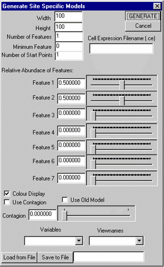
- The following are the constraints that can be used to express a site model:
- i) Width: The number of columns (cells per row) in the site model raster.
- ii) Height: The number of rows (cells per column) in the site model raster.
- iii) Number of Features: The maximum number of features (landscape element types) that may occur in an instance.
- iv) Minimum Feature: The numeric value of the first feature (generally 0 or 1).
- v) Number of Start Points: This is used in conjunction with contagion. It specifies the number of locations that are to be independently chosen (i.e. without using contagion). It must be at least one, but may be any positive number. These points are selected randomly in the output map. The remaining cells are produced using the influence of contagion and previously computed cell values.
- vi) Cell Expression: The file name of a cell expression to evaluate for computing the site-specific relative probabilities.
- vii) Relative Abundance of Features: The site independent relative abundance (i.e. relative probability) of each of the first seven features. These represent the expected relative occurrence of each feature in the landscape, in the absence of other spatial information. At a given site, the relative probabilities returned by the cell expression are multiplied by these static probabilities to produce a final set of relative probabilities for the site. Where contagion is used (especially high values of contagion), the actual abundance may be quite different. In this situation, these represent the expected relative occurrence of each feature over all instances of the model. Note that the relative abundance specified for feature 7 applies to all features greater than 7 (i.e. it applies to features in the range [7, Number of Features].
- viii) Colour Display: If selected, then instances will be displayed in colour. Otherwise they will be displayed in black and white.
- ix) Use Contagion: If selected, then contagion is used to generate model instances. Contagion represents the degree to which features in the landscape are grouped together. A contagion value of 0 means no contagion (i.e. adjacency of features is random), while a value of 1 means that the probability of adjacent cells having the same value is 1. Values of contagion between zero and one cause varying degrees of "clumping" or spatial autocorrelation.
- x) Contagion: The value of contagion to use. Currently, the value can only be in the range [0,1].
- xi) Use Old Model: If selected, produce model instances using an older algorithm. The older algorithm exhibits a "stripping" bias when high levels of contagion are specified.
- xii) Variable and Viewname drop-down lists: the names of the views (windows) for layer variables used by the cell expression. For example, if the cell expression requires a layer variable called “topography”, then this variable will appear in the Variables list. This will map to view that contains topography in the Viewnames list.
- xiii) Load from File/Save to File: Load model parameters from or save to the file specified in the adjacent text box. These files generally should have a .sm suffix. It is useful to load pre-existing model files, modify them to suit the current needs and then save these to a new file. These site model files can be opened directly using the Open menu item in the Files menu described in section II.

- d) Value (or Statistical Summary) Model: Value (or summary) models produce a single value by summarizing a function (specified as a cell expression) that computes a value for each cell in the landscape. The resulting value is displayed in the dialog box when “Generate” is pressed.
- To compute a value model, set up the function, as described below, and press the Run button to compute from an input file or RunEdits to compute from the expression written in the edit box. When finished, the dialog can be close with the Cancel button.
- The following parameters can be used to express a value model:
- i) Operation: Chose the desired summary function: mean, minimum value, maximum value, sum over all values, product over all values, nth root over all values (where n is the number of values computed).
- ii) Cell Expression: The file name of a cell expression to evaluate for computing the value for each site.
- iii) Region: The region is always the entire landscape. The edit box associated with the region allows users to specify a decision to limit the computation to a specific portion of the landscape.
- iv) Variable and Viewname drop-down lists: the names of the views (windows) for layer variables used by the cell expression. For example, if the cell expression requires a layer variable called “topography”, then this variable will appear in the Variables list. This will map to view that contains topography in the Viewnames list. When opened, all current views are automatically linked to variables of the same name.
- v) Cell Expression Edit box: This box allows users to type in an arbitrary cell expression, and can be used much like a console for querying or modifying the landscape state.
- e) Align Layer: The Align Layer feature aligns the currently selected layer with the layer chosen in the “Align with Layer” drop-down list by matching their georeferencing. If the layers are already aligned, no action is performed. If the layers are not aligned, then a new view is created with the name “alignedMAP”, where "MAP" is the name of the view chosen to align. The georeferencing of the new view will match the view chosen in the “Align with Layer” drop-down list. The contents of the new view will be the original view clipped to the new georeferencing. Any cells within the clip region, but not covered by the original layer will have a value of zero.
- Models in SELES must be aligned to run properly. That is, all raster layers must have the same extent (number of rows and columns) and must represent the same geographic location. This permits simulations to access all relevant information for a cell with a single location index.
- Once the layer to align with has been selected, the top-left and bottom-right bounds of the original image are shown relative to the georeferencing of the “Align with Layer”. These are called the aligned bounds. Any portion of the layer outside the range of the "Align with Layer" is clipped. Once an appropriate "Align with Layer" has been selected, the operation is performed by pressing the OK button.
- f) Resize Layer: The Resize Layer feature allows a raster to be resized, without changing its resolution. The dialog allows users to enter new bounds (top, left, bottom, right) for the raster. When the OK button is pushed, a new view with the same name but prefixed with “Resized” is created for the resized raster.
Dynamic Models Menu
There are three types of dynamic models available from this menu, a dialog box for setting up dynamic output of layers, and a dialog box for controlling simulations. Dynamic models generally produce a series of model instances or, in the case of Dynamic Value Models, a series of values, during the course of a simulation. All three dynamic models (Dynamic Site Model, Dynamic Value Model, Seles Model) may depend on other layers in the current scenario.
- a) Dynamic Site Model: A Dynamic Site Model is a site model that is re-computed periodically during a simulation. Since these models may depend on dynamically changing layers in the scenario, periodic recomputation of the model may produce different results.
- The dialog is identical to the static Site Model dialog except for an “Output Frequency” option. The value specified (in days and years) determines how often the site model is to be recomputed. For example, a value of 2 years will cause the model to be recomputed every 730.5 days or unit time steps. If the output frequency is zero, then the site model will be recomputed every time an event occurs during the simulation. If the output frequency is negative, then the model will be recomputed every time one of the parameter layers is modified. This may be useful if one or more of the parameter layers are being changed by an external model.
- b) Dynamic Value Model: A Dynamic Value Model is a value model that is re-computed periodically during a simulation. Since these models may depend on one or more dynamically changing layers in the scenario, periodic updating may produce different results. The dialog is similar to the static Value Model dialog with two additional options.
- i) Output Filename: If the “Save Output to File” option is chosen, then the output will be stored in the named file. Each run (of a Monte Carlo simulation) will be stored on a different line, and each output value will be separated by a tab character. This allows the model output to be loaded into a spreadsheet (e.g. Excel) for post-mortem analysis.
- ii) Output Frequency: The value specifies how often the model is to be recomputed during a simulation. If the output frequency is zero, then the model will be recomputed every time an event occurs during the simulation. If the output frequency is negative, then the model will be recomputed every time one of the parameter layers is modified.

- c) Model Output: Model Output allows intermediate states of dynamic layers to be saved during a simulation. The "Output Frequency" species how often the currently selected layer is to be saved. Each time the raster layer is saved, a new file is created with a unique filename: "BaseName#r.#s", where "BaseName" is the base filename, "#r" is the Monte Carlo run number, and "#s" is the sequence number for layer in this run. The “Filename Base or Directory” specifies where the raster layers are to be saved. If this names an existing directory, then the name of the currently selected layer will be used as the base filename, otherwise it specifies the full path and filename to be used as the base filename. For example, during run 2 with a filename base of “./results/test”, the sequence of files will be: './results/test2.1', './results/test2.2', etc. The available output types are uncompressed and compressed GRASS binary and GRASS ASCII, ERDAS 8 and 16 bit and ARC ASCII. Model output is set up by pressing the OK button, and terminated by pressing the Stop Output button.

- d) Seles Model: A SELES Model specifies the information required to set up a simulation: that is, the input layers (initial spatial state), output layers (dynamic spatial state) and the landscape events. Once the information is entered or modified in the dialogue box, press “Setup” to prepare the model for simulation. This will not start a simulation – this is done using the Simulation Control dialog.
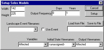
- The following parameters are used to express a SELES model:
- i) Width and Height: Specifies the spatial resolution as the number of columns and rows in the raster layers used by the scenario.
- ii) Output Frequency: The default frequency with which dynamic layers are updated on the screen. If the output frequency is zero, then the view for the dynamic layers will be refreshed every time an event occurs during a simulation.
- iii) Landscape Event Filenames: A drop-down list of the file names of landscape events used in the simulation. A SELES simulation requires one or more landscape events. The “Use Event” check box can be used to disable/enable specific events.
- iv) Variables and Initial State Viewnames: There is a (partial) mapping from layer variables in landscape events to viewnames that contain the initial spatial state of the variable. This mapping connects variables with their starting state raster layers at the beginning of a simulation or Monte-Carlo run. If the viewname is “<unassigned>”, then the initial state is assume to be a raster of zeros.
- v) Variables and Output Viewnames: There is a (partial) mapping from dynamic layer variables in landscape events to viewnames that contain the current (dynamic) spatial state of the variable. This mapping connects variables with the view in which the dynamic output layer for this variable is displayed during a simulation. If the viewname is “<unassigned>”, then the output state is not displayed (but will be maintained internally).
- vi) Load from File/Save to File: Load model parameters from or save to the file specified in the adjacent text box. These files generally should have a .sel suffix. It is useful to load pre-existing model files, modify them to suit the current needs and then save these to a new file. These SELES model files can be opened directly using the Open menu item in the Files menu described in section II.

- e) Simulate: This displays a dialog that provides the necessary functions to control simulations. Once all the dynamic models are set up, then the simulation scenario is ready to run. Since this dialog is modeless, other actions can be performed while the box is on the screen, and while a simulation is in progress.
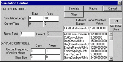
- The dialog allows control of a simulation as follows:
- i) Simulation Length: Specifies (in days and years) the length of time to run a simulation. “Current Time” is an output value that shows the current time of a running simulation. Note that a SELES model may use any unit timestep. For convenience, the unit timestep is called a "day" on the user interface, where one year = 365.25 days. If the unit timestep in your model is not a day, then read "Days" as "Unit Timesteps" on SELES dialogues.
- ii) Runs: Total: Specifies the number of Monte Carlo simulation runs. This can only be set before a simulation starts. “Runs: Current” is an output value that shows the current Monte Carlo run number.
- iii) Output Frequency: Specifies how often the model in the currently selected view is to be redisplayed. (See notes on unit timestep above.)
- iv) Step Size: Specifies how the number of time-steps to be made when “stepping through” a simulation.
- v) Simulate: Starts a simulation (or a complete series of Monte Carlo simulations). This button will change to a “Stop” during the simulation. Pressing “Stop” will terminate the simulation.
- vi) Pause: Allows a simulation to pause. While on pause, this button will change to a “Continue” button. Pressing “Continue” will resume the simulation.
- vii) Step: Allows a simulation to be "stepped through" in discrete time steps. If the simulation has not yet begun, then pressing this button will start it. Once the time period specified by “Step Size” has passed, the simulation will pause. At this point the “Pause” button will change to “Continue”. The user can press “Step” again to continue the simulation for “Step Size” time units, or press “Continue” to continue the simulation without stepping. Note that the Step button can be pressed at any time during a simulation to enter step mode.
- viii) Cancel: If a simulation is currently running, Cancel is the same as Stop. If a simulation is not running, then Cancel will close the Simulation Control Dialog.
- ix) External Global Variables: This is a list of global variables defined in landscape events. The initial state value of global variables is zero by default, but may be specified in a SELES Model file or dialogue. During a simulation, the values of dynamic variables are periodically updated in the dialog box. The current value of a global variable can be changed by selecting it in the scrollable list, typing a new value in the “Value” edit box and pressing “Set”. The initial state value of a variable can be similarly changed, pressing “Set Initial State” instead of “Set”.

- f) Simulation Probe: This option brings up a dialog box that allows probing of internal values in landscape events/agents during simulation. The desired event can be selected from a drop-down menu as well as the desired property context. Values for the agent/cell, cluster/group, event/population and cell variables are shown in different areas of the dialog. If changes occur too fast to see, there is an option to slow down the simulation. Care must be taken when using the probe, since it must modify events to operate. As a consequence, making too many changes on the dialog runs the risk of crashing a simulation due to timing of the user interface operation and the separate simulation engine processes.
- g) Model Report: This option saves a dynamic model report to two files called “SelesModelReport.txt” and “SelesModelReport2.txt” in the current directory. These files organizes all the layer and global variables, and global constants in the model state-space by type and lists the events that include them in their definitions section. The files also indicate if a variable or constant appears on the left-hand side (LHS), right-hand side (RHS), both or neither of an expression in the named event. The only difference between the files is format – the first is easier for browse while the second is more suitable for loading into a spreadsheet. This is useful for model verification, since at a glance it is easy to see variables that are not used, misspelled or not declared properly. Particular attention should be paid to variables that have no initial state.
- h) Simulation Priority: This option allows users to set the priority level for the simulation engine. On a single-processor machine (i.e. most desktops and laptops), decreasing the engine priority to Low or Lowest can increase responsiveness of the user interface and other programs.